Word Embeddings and Vector Semantics

Welcome to Word Embeddings!

What You’ll Learn

By the end of this tutorial, you will be able to:

• Understand what word embeddings are and why they revolutionized NLP
  
• Grasp the distributional hypothesis: “You shall know a word by the company it keeps”
  
• Train your own word2vec models from text data
  
• Use pre-trained embeddings (GloVe, fastText, BERT)
  
• Find similar words using vector mathematics
  
• Perform word analogies (king - man + woman = queen)
  
• Visualize embeddings in 2D space
  
• Apply embeddings to real research questions
  
• Understand when to use which embedding method
  

What Are Word Embeddings?

Word embeddings are dense vector representations of words that capture semantic meaning. Instead of representing words as arbitrary symbols, embeddings place semantically similar words near each other in a multi-dimensional space.

The Problem with Traditional Approaches

One-hot encoding (traditional approach):

cat  = [1, 0, 0, 0, 0, ..., 0]  (10,000 dimensions)  
dog  = [0, 1, 0, 0, 0, ..., 0]  
car  = [0, 0, 1, 0, 0, ..., 0]  

Problems:
- No semantic relationship captured
- “cat” is as different from “dog” as from “car”
- Extremely sparse (mostly zeros)
- Vocabulary size = dimensions
- No generalization

Word embeddings (modern approach):

cat  = [0.2, -0.4, 0.7, ..., 0.1]  (300 dimensions)  
dog  = [0.3, -0.5, 0.8, ..., 0.2]  (similar to cat!)  
car  = [-0.1, 0.6, -0.3, ..., 0.4] (different from cat/dog)  

Advantages:
- ✅ Semantic similarity captured
- ✅ Dense, efficient representation
- ✅ Fixed dimensions (typically 50-300)
- ✅ Enables generalization
- ✅ Mathematical operations meaningful

The Distributional Hypothesis

“You shall know a word by the company it keeps” — J.R. Firth (1957)

Core idea: Words appearing in similar contexts have similar meanings.

Example:
- “The cat sat on the mat”
- “The dog sat on the mat”
- “The car drove down the street”

Words like “cat” and “dog” appear in similar contexts (sat, mat) → should have similar embeddings.

Why Word Embeddings Matter

Revolution in NLP

Before embeddings (pre-2013):
- Manual feature engineering
- Bag-of-words models
- No semantic understanding
- Poor generalization

After embeddings (2013+):
- Automatic feature learning
- Rich semantic representations
- Captures analogies and relationships
- Transfer learning possible

Real-World Applications

Application	How Embeddings Help
Search engines	Find semantically similar documents
Machine translation	Map words across languages
Sentiment analysis	Understand emotional content
Question answering	Match questions to answers semantically
Text classification	Better features for ML models
Information retrieval	Go beyond keyword matching
Recommendation systems	Find similar items/content
Named entity recognition	Recognize entities in context

Linguistic Research Applications

Semantic change detection:
- Track meaning shifts over time
- Compare embeddings from different decades
- Study language evolution

Bias detection:
- Uncover implicit associations
- Gender bias (doctor → male, nurse → female)
- Racial bias in language models

Metaphor analysis:
- Identify non-literal meanings
- Cross-domain mappings
- Conceptual structures

Dialect/register variation:
- Compare vocabulary usage
- Identify characteristic terms
- Study sociolinguistic patterns

Tutorial Citation

Schweinberger, Martin. 2026. Word Embeddings and Vector Semantics. Brisbane: The Language Technology and Data Analysis Laboratory (LADAL). url: https://ladal.edu.au/tutorials/embeddings.html (Version 2026.02.08).

Prerequisites

Before starting, familiarize yourself with:

• Getting started with R
• Text processing in R
• Basic statistics
• Basic understanding of vectors and matrices

---

Part 1: Understanding Embeddings

Vector Space Models

The Core Concept

Embeddings represent words as vectors in high-dimensional space where:
- Each dimension captures some aspect of meaning
- Similar words cluster together
- Relationships are preserved geometrically

Simplified 2D example:

         happy •  
               |  
    joyful •   |   • excited  
               |  
    -----------+----------- (dimension 1)  
               |  
         sad • |  
               |  
               (dimension 2)  

In reality: 50-300 dimensions, not 2!

Mathematical Properties

Distance measures similarity:

# Cosine similarity (most common)  
similarity = (A · B) / (||A|| × ||B||)  
  
# Range: -1 (opposite) to +1 (identical)  

Vector arithmetic works:

king - man + woman ≈ queen  
Paris - France + Germany ≈ Berlin  

This is remarkable — mathematical operations on word vectors produce meaningful semantic results!

Types of Word Embeddings

1. Count-Based Methods (Classical)

Co-occurrence matrix:
- Count how often words appear together
- Apply dimensionality reduction (SVD)
- Examples: LSA, HAL

Advantages:
- Straightforward to understand
- Interpretable dimensions
- Good for small datasets

Disadvantages:
- Computationally expensive for large vocabularies
- Sparse matrices
- Less effective than modern methods

2. Prediction-Based Methods (Modern)

Neural network models:
- Predict context from word or word from context
- Learn embeddings as model weights
- Examples: word2vec, GloVe, fastText

Two main architectures:

CBOW (Continuous Bag of Words):
- Input: Context words
- Output: Target word
- Fast training
- Better for frequent words

Skip-gram:
- Input: Target word
- Output: Context words
- Slower training
- Better for rare words and small datasets

Advantages:
- Capture nuanced semantics
- Efficient for large datasets
- State-of-the-art performance

3. Contextualized Embeddings (Cutting-Edge)

Context-dependent representations:
- Same word, different embeddings in different contexts
- Examples: ELMo, BERT, GPT

Example:

"Bank" in "river bank" ≠ "Bank" in "savings bank"  

Traditional embeddings: one vector for “bank”
Contextualized: different vectors based on context

We’ll focus primarily on word2vec and GloVe (most widely used for linguistic research), with guidance on when to use contextualized models.

The word2vec Algorithm

How It Works

Training objective: Given a word, predict its context (or vice versa)

Skip-gram example:

Sentence: “The quick brown fox jumps”
Target word: “brown”
Window size: 2

Training pairs:
- (brown, the)
- (brown, quick)
- (brown, fox)
- (brown, jumps)

The neural network learns to predict these context words from “brown”, adjusting the embedding to maximize prediction accuracy.

Training Process

1. Initialize random vectors for all words
   
2. For each word in corpus:
   • Get context words (within window)
     
   • Predict context using current embeddings
     
   • Calculate prediction error
     
   • Update embeddings to reduce error
     
3. Repeat until convergence

Result: Words with similar contexts end up with similar vectors!

Key Hyperparameters

Parameter	What It Controls	Typical Values	Effect
vector_size	Embedding dimensions	50-300	Higher = more nuance, slower
window	Context size	5-10	Larger = broader semantics
min_count	Min word frequency	5-10	Filters rare words
sg	Skip-gram (1) or CBOW (0)	0 or 1	Skip-gram better for small data
negative	Negative samples	5-20	Optimization technique
epochs	Training iterations	5-50	More = better learning (to a point)

Training Trade-offs

Bigger isn’t always better:
- More dimensions: captures subtleties but risks overfitting
- Larger window: broader semantic relationships but less specific
- More epochs: better learning but diminishing returns

Best practice: Start with defaults, then experiment systematically.

---

Part 2: Setup and Installation

Required Packages

# Core embedding packages  
install.packages("word2vec")      # Train word2vec models  
install.packages("text2vec")      # Alternative implementation  
install.packages("wordVectors")   # Load/manipulate embeddings  
  
# Pre-trained embeddings  
install.packages("textdata")      # Download GloVe  
  
# Manipulation and analysis  
install.packages("dplyr")         # Data wrangling  
install.packages("stringr")       # String processing  
install.packages("tidyr")         # Data reshaping  
install.packages("purrr")         # Functional programming  
  
# Visualization  
install.packages("ggplot2")       # Plotting  
install.packages("ggrepel")       # Better text labels  
install.packages("Rtsne")         # Dimensionality reduction  
install.packages("umap")          # Alternative to t-SNE  
  
# Utilities  
install.packages("here")          # File paths  
install.packages("flextable")     # Tables  

Loading Packages

# Load packages  
library(word2vec)  
library(text2vec)  
library(dplyr)  
library(stringr)  
library(tidyr)  
library(purrr)  
library(ggplot2)  
library(ggrepel)  
library(Rtsne)  
library(here)  
library(flextable)  

Package Ecosystem

• word2vec: Easiest for beginners, good documentation
  
• text2vec: More advanced, faster for large datasets
  
• wordVectors: Excellent for loading pre-trained models
  
• textdata: Easy access to GloVe embeddings

We’ll primarily use word2vec for training and textdata for pre-trained models.

---

Part 3: Training Your First Model

Loading Example Data

We’ll use a collection of texts to train our embedding model. For this tutorial, we’ll use literary texts that provide rich semantic content.

# Load example texts (Alice's Adventures in Wonderland, Moby Dick, Pride and Prejudice)  
# In practice, you'd load your own corpus  
alice <- readLines(here::here("tutorials/embeddings/data", "alice.txt"))  
moby <- readLines(here::here("tutorials/embeddings/data", "moby.txt"))
pride <- readLines(here::here("tutorials/embeddings/data", "pride.txt"))

# Combine into single corpus  
corpus <- paste(c(alice, moby, pride), collapse = " ")
  
# Basic preprocessing  
corpus_clean <- corpus |>  
  tolower() |>                              # lowercase  
  str_replace_all("\\s+", " ") |>           # normalize whitespace  
  str_trim()                                 # trim edges  
  
# Inspect  
cat("Corpus size:", str_count(corpus_clean, "\\S+"), "words\n")  

Corpus size: 362385 words

cat("First 200 characters:\n")  

First 200 characters:

cat(substr(corpus_clean, 1, 200), "...\n")  

*** start of the project gutenberg ebook 11 *** [illustration] alice’s adventures in wonderland by lewis carroll the millennium fulcrum edition 3.0 contents chapter i. down the rabbit-hole chapter ii. ...

Preprocessing Considerations

For embeddings, you might want to:
- Keep punctuation if studying syntax
- Preserve case for named entities
- Remove or keep numbers (depends on task)
- Handle contractions consistently

Our simple approach: Lowercase, remove punctuation, normalize spaces. Adjust based on your research questions!

Training a word2vec Model

Basic Training

Critical: Text Format for word2vec

The word2vec function requires tokenized text - either:
1. A character vector where each element is a sentence
2. A data frame with sentences in rows

It does NOT work with a single long string!

# IMPORTANT: Split into sentences for word2vec  
# The function needs sentences as separate elements  
corpus_sentences <- corpus_clean |>  
  # Split into sentences (simple approach using periods)  
  str_split("\\.\\s+") |>  
  unlist() |>  
  # Remove empty sentences  
  discard(~ nchar(.x) == 0)  
  
# Train model  
model <- word2vec(  
  x = corpus_sentences,      # Tokenized as sentences!  
  type = "skip-gram",        # Skip-gram architecture  
  dim = 100,                 # 100-dimensional vectors  
  window = 5,                # 5-word context window  
  iter = 20,                 # 20 training iterations  
  min_count = 5,             # Ignore words appearing < 5 times  
  threads = 2                # Use 2 CPU threads  
)  
  
# Inspect model  
summary(model)[1:50]        # show first 50 terms

 [1] "abundantly"   "acceptance"   "accompany"    "accounting"   "ache"        
 [6] "adhering"     "afar"         "aged"         "alacrity"     "alien"       
[11] "altar"        "amazed"       "amber"        "amends"       "anatomical"  
[16] "anchored"     "andes"        "animation"    "answers"      "antarctic"   
[21] "antique"      "apologize"    "apple"        "apply"        "arrested"    
[26] "arrow"        "artificial"   "ascribed"     "assertion"    "associations"
[31] "assuming"     "atmosphere"   "attacked"     "attempts"     "attractions" 
[36] "attribute"    "attributed"   "augment"      "authorities"  "axe"         
[41] "bade"         "banished"     "barb"         "barely"       "bats"        
[46] "beard"        "befell"       "behalf"       "bingleys"     "bitterly"    

What just happened:
1. Text split into words
2. Neural network initialized
3. For each word, model learns to predict context
4. Embeddings adjusted over 20 iterations
5. Final word vectors saved in model

Exploring the Model

# Get vocabulary  
vocabulary <- summary(model$vocabulary)  
  
# Inspect vocabulary size  
cat("Vocabulary size:", length(vocabulary), "words\n")  

Vocabulary size: 6 words

# Most common words  
head(vocabulary[order(-vocabulary)], 20)  

   Min. 1st Qu.  Median    Mean 3rd Qu.    Max. 
   5876    5876    5876    5876    5876    5876 

Extracting Embeddings

# Get embedding matrix  
embedding_matrix <- as.matrix(model)  
  
# Inspect dimensions  
cat("Embedding matrix:", nrow(embedding_matrix), "words ×",   
    ncol(embedding_matrix), "dimensions\n")  

Embedding matrix: 5876 words × 100 dimensions

# Look at a specific word  
word_example <- "alice"  
if (word_example %in% rownames(embedding_matrix)) {  
  cat("\nEmbedding for '", word_example, "':\n", sep = "")  
  cat(embedding_matrix[word_example, 1:10], "...\n")  
}  

Embedding for 'alice':
-1.341396 -0.4444789 -0.06832235 0.3490041 0.06123342 0.6413595 -0.4662222 -0.1370008 0.1918846 1.062878 ...

Interpretation:
- Each row = one word
- Each column = one dimension of meaning
- Values are learned weights
- Similar words have similar patterns

---

Part 4: Finding Similar Words

Semantic Similarity

The most immediate use of embeddings: finding words with similar meanings.

Most Similar Words

# Find words similar to "queen"  
similar_to_queen <- predict(  
  model,   
  newdata = c("queen"),   
  type = "nearest",  
  top_n = 10  
)  
  
# Display results  
similar_to_queen |>  
  as.data.frame() |>  
  flextable() |>  
  set_table_properties(width = .5, layout = "autofit") |>  
  theme_zebra() |>  
  set_caption("Top 10 words most similar to 'queen'") |>  
  border_outer()  

queen.term1	queen.term2	queen.similarity	queen.rank
queen	knave	0.7576630	1
queen	king	0.7342355	2
queen	“here	0.7292620	3
queen	hatter	0.7288208	4
queen	mouse	0.7159314	5
queen	executioner	0.7064495	6
queen	hare	0.7058222	7
queen	duchess	0.7039048	8
queen	alice	0.7006320	9
queen	dormouse	0.6982160	10

How similarity is calculated:

cosine_similarity = (A · B) / (||A|| × ||B||)  

Where:
- A, B are word vectors
- · is dot product
- || || is vector magnitude
- Result ranges from -1 (opposite) to 1 (identical)

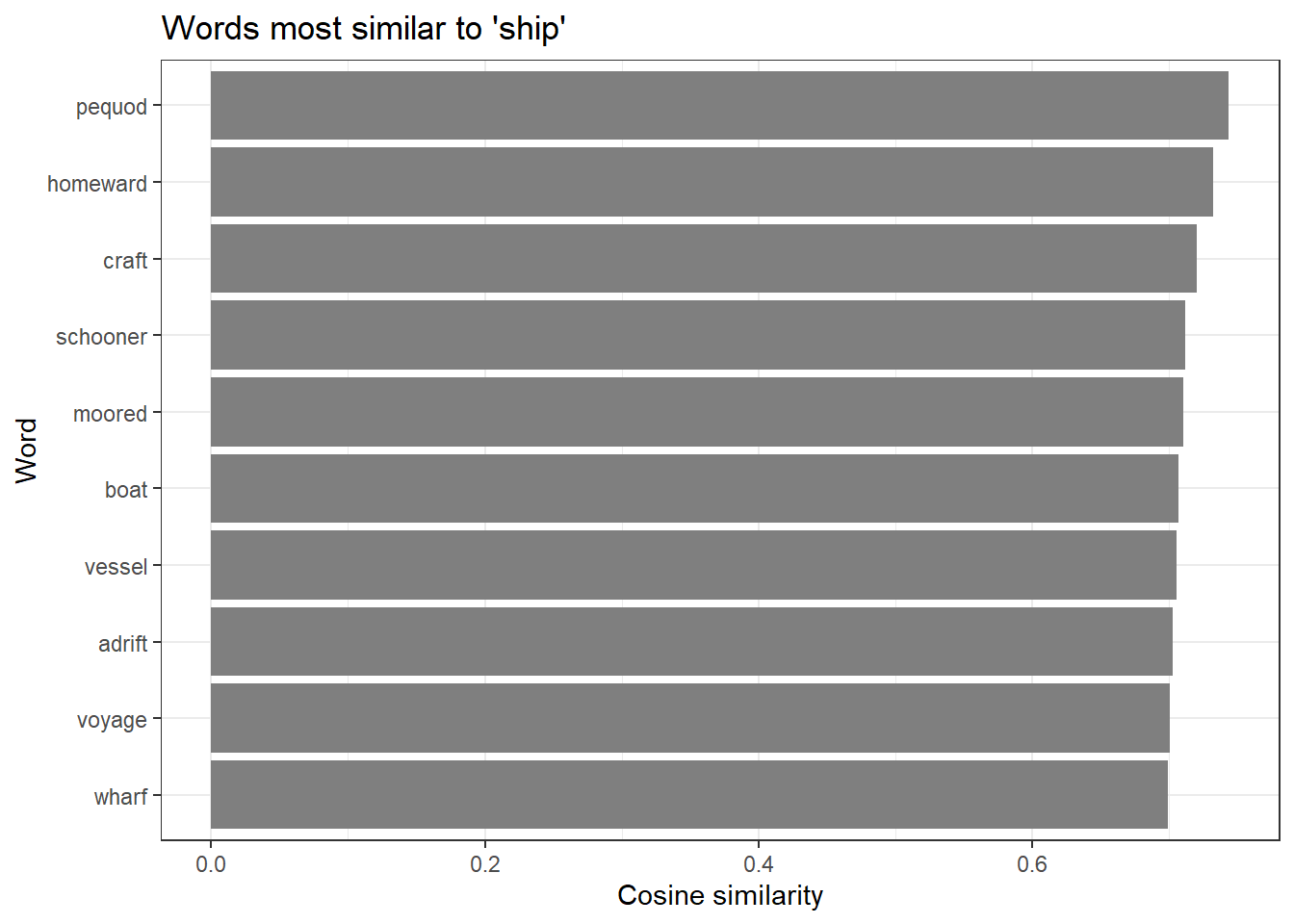
Exploring Different Words

# Try multiple words  
test_words <- c("love", "king", "ocean", "thought")  
  
for (word in test_words) {  
  if (word %in% rownames(embedding_matrix)) {  
    similar <- predict(model, newdata = word, type = "nearest", top_n = 5)  
    cat("\nMost similar to '", word, "':\n", sep = "")  
    print(as.data.frame(similar)[1:5,2])  
  }  
}  

Most similar to 'love':
[1] "girl"      "earnest"   "gratitude" "marry"     "consent"  

Most similar to 'king':
[1] "queen"       "executioner" "angrily"     "rome"        "x"          

Most similar to 'ocean':
[1] "floated"  "seas"     "japanese" "fold"     "lone"    

Most similar to 'thought':
[1] "grieved"      "guessed"      "recollecting" "won"          "“shall"      

Interpreting Similarity Results

What makes words similar:
- Semantic relatedness (synonyms, related concepts)
- Grammatical function (both nouns, both verbs)
- Topical association (co-occur in same contexts)

Not just synonyms!
- “king” and “queen” are similar (related roles)
- “ocean” and “sea” are similar (synonyms)
- “love” and “hate” might be similar (both emotions, appear in similar contexts)

Similarity Scores

# Get similarity with scores  
similar_with_scores <- predict(  
  model,  
  newdata = c("ship"),  
  type = "nearest",  
  top_n = 15  
)  
  
# Visualize  
similar_with_scores |>  
  as.data.frame() |>  
  head(10) |>  
  ggplot(aes(x = reorder(ship.term2, ship.similarity), y = ship.similarity)) +
  geom_bar(stat = "identity", fill = "steelblue") +  
  coord_flip() +  
  labs(  
    title = "Words Similar to 'ship'",  
    x = "Word",  
    y = "Cosine Similarity"  
  ) +  
  theme_minimal()  

Reading the plot:
- Higher bars = more similar
- Similarity typically 0.3-0.9 for related words
- Top words share contexts with target word

---

Part 5: Word Analogies

Vector Arithmetic

One of the most fascinating properties: algebraic operations on word vectors preserve semantic relationships.

The Classic Example

king - man + woman ≈ queen

Since the word2vec package doesn’t have built-in analogy functionality, we’ll compute it manually using vector arithmetic.

# Helper function to compute word analogies  
# Computes: a is to b as c is to ?  
# Mathematically: result ≈ b - a + c  
word_analogy <- function(model, a, b, c, top_n = 5) {  
  # Get embedding matrix  
  embeddings <- as.matrix(model)  
    
  # Check all words exist  
  if (!all(c(a, b, c) %in% rownames(embeddings))) {  
    missing <- c(a, b, c)[!c(a, b, c) %in% rownames(embeddings)]  
    stop(paste("Words not in vocabulary:", paste(missing, collapse = ", ")))  
  }  
    
  # Get word vectors  
  vec_a <- embeddings[a, ]  
  vec_b <- embeddings[b, ]  
  vec_c <- embeddings[c, ]  
    
  # Compute target vector: b - a + c  
  target_vector <- vec_b - vec_a + vec_c  
    
  # Calculate cosine similarity with all words  
  similarities <- apply(embeddings, 1, function(word_vec) {  
    # Cosine similarity  
    sum(word_vec * target_vector) /   
      (sqrt(sum(word_vec^2)) * sqrt(sum(target_vector^2)))  
  })  
    
  # Remove the input words from results  
  similarities <- similarities[!names(similarities) %in% c(a, b, c)]  
    
  # Get top N most similar  
  top_words <- sort(similarities, decreasing = TRUE)[1:top_n]  
    
  # Return as dataframe  
  result <- data.frame(  
    word = names(top_words),  
    similarity = as.numeric(top_words),  
    row.names = NULL  
  )  
    
  return(result)  
}  

# Perform word analogy: man is to king as woman is to ?  
# Mathematically: king - man + woman  
analogy_result <- word_analogy(  
  model,  
  a = "man",  
  b = "king",   
  c = "woman",  
  top_n = 5  
)  
  
# Display  
analogy_result |>  
  flextable() |>  
  set_table_properties(width = .5, layout = "autofit") |>  
  theme_zebra() |>  
  set_caption("king - man + woman = ?") |>  
  border_outer()  

word	similarity
civilities	0.4407494
queen	0.4366286
defects	0.4246290
impatiently	0.4151644
console	0.4123673

Expected result: “queen” should be top or near top (depending on corpus quality).

How It Works

Mathematical operation:

target_vector = embedding("king") - embedding("man") + embedding("woman")  
result = find_nearest(target_vector)  

Geometric interpretation:
1. Vector from “man” to “king” represents royalty/leadership
2. Apply same transformation to “woman”
3. Result should be female royalty

Step-by-step:

# 1. Get the "royalty" direction  
royalty_vector = king - man  
  
# 2. Apply to "woman"  
target = woman + royalty_vector  
  
# 3. Which equals  
target = woman + (king - man) = king - man + woman  

More Analogies

# Try different analogies if words exist in vocabulary  
  
# Test if words exist first  
vocab <- rownames(as.matrix(model))  
  
# Example 1: Tense (if available)  
if (all(c("walking", "walk", "running") %in% vocab)) {  
  cat("walking : walk :: running : ?\n")  
  result <- word_analogy(model, "walk", "walking", "running", top_n = 3)  
  print(result$word[1:3])  
  cat("\n")  
}  

walking : walk :: running : ?
[1] "pulled"  "king’s"  "jumping"

# Example 2: Comparative/superlative (if available)    
if (all(c("good", "better", "bad") %in% vocab)) {  
  cat("good : better :: bad : ?\n")  
  result <- word_analogy(model, "good", "better", "bad", top_n = 3)  
  print(result$word[1:3])  
  cat("\n")  
}  

good : better :: bad : ?
[1] "tricks"  "—that’s" "belongs"

# Example 3: Same relationship in different domain  
if (all(c("alice", "wonderland", "dorothy") %in% vocab)) {  
  cat("alice : wonderland :: dorothy : ?\n")  
  result <- word_analogy(model, "alice", "wonderland", "dorothy", top_n = 3)  
  print(result$word[1:3])  
  cat("\n")  
}  

Analogy Limitations

Analogies work best when:
- Relationship is consistent in training data
- All words appear frequently enough
- Relationship is “regular” (not idiomatic)
- Corpus is large (10M+ words)

Common failures:
- Small corpus (like our Alice example)
- Idioms and irregular forms
- Cultural-specific knowledge
- Subtle semantic distinctions

Not magic! Analogies reflect patterns in your training data, including biases and inconsistencies. With Alice in Wonderland alone, we won’t get perfect analogies - you’d need much larger, more diverse text.

Custom Analogies

# Function to test analogies with better error handling  
test_analogy <- function(model, a, b, c, label = NULL) {  
  if (is.null(label)) {  
    label <- paste(a, ":", b, "::", c, ": ?")  
  }  
    
  vocab <- rownames(as.matrix(model))  
    
  # Check if all words in vocabulary  
  if (!all(c(a, b, c) %in% vocab)) {  
    missing <- c(a, b, c)[!c(a, b, c) %in% vocab]  
    cat(label, "\n")  
    cat("ERROR: Words not in vocabulary:", paste(missing, collapse = ", "), "\n\n")  
    return(NULL)  
  }  
    
  result <- word_analogy(model, a, b, c, top_n = 5)  
    
  cat(label, "\n")  
  cat("Top results:", paste(result$word[1:5], collapse = ", "), "\n")  
  cat("Similarities:", paste(round(result$similarity[1:5], 3), collapse = ", "), "\n\n")  
    
  return(result)  
}  
  
# Try several (may fail with small corpus)  
test_analogy(model, "queen", "woman", "man", "queen : woman :: man : ?")  

queen : woman :: man : ? 
Top results: person, tribe, education, young, picture 
Similarities: 0.443, 0.44, 0.425, 0.422, 0.42 

       word similarity
1    person  0.4431919
2     tribe  0.4396194
3 education  0.4248894
4     young  0.4222039
5   picture  0.4197212

test_analogy(model, "alice", "girl", "boy", "alice : girl :: boy : ?")  

alice : girl :: boy : ? 
Top results: spoiled, healthy, coward, sweetest, where’s 
Similarities: 0.536, 0.473, 0.445, 0.426, 0.417 

      word similarity
1  spoiled  0.5364251
2  healthy  0.4732269
3   coward  0.4449884
4 sweetest  0.4263174
5  where’s  0.4169461

# You can add your own  
# test_analogy(model, "word1", "word2", "word3")  

Getting Better Analogies

For impressive analogy results, you need:

1. Large, diverse corpus (100M+ words ideal)
- Use pre-trained embeddings (GloVe, fastText)
- Or train on Wikipedia, news corpora, books corpus

2. Higher-frequency words
- Words appearing 1000+ times work best
- Rare words have noisier embeddings

3. Consistent relationships
- “Gender” works well (man/woman, king/queen)
- “Geography” works well (capital cities)
- Grammatical relationships work well (tense, number)

Try with pre-trained embeddings:

# Using pre-trained GloVe (see Part 7)  
# You'll get much better analogy results!  

Visualizing Vector Arithmetic

Let’s visualize what’s happening geometrically:

# Only run if we have the key words  
vocab <- rownames(as.matrix(model))  
  
if (all(c("man", "woman", "king", "queen") %in% vocab)) {  
  # Get embeddings  
  embeddings <- as.matrix(model)  
    
  # Get specific words  
  words_of_interest <- c("man", "woman", "king", "queen")  
  word_embeddings <- embeddings[words_of_interest, ]  
    
  # Reduce to 2D with PCA for visualization  
  pca_result <- prcomp(word_embeddings, center = TRUE, scale. = FALSE)  
    
  # Create dataframe  
  viz_data <- data.frame(  
    word = words_of_interest,  
    x = pca_result$x[, 1],  
    y = pca_result$x[, 2]  
  )  
    
  # Plot  
  ggplot(viz_data, aes(x = x, y = y, label = word)) +  
    geom_point(size = 4, color = "steelblue") +  
    geom_text_repel(size = 5, fontface = "bold") +  
    geom_segment(aes(x = x[1], y = y[1], xend = x[3], yend = y[3]),  
                 arrow = arrow(length = unit(0.3, "cm")),   
                 color = "red", linewidth = 1,  
                 data = viz_data[viz_data$word %in% c("man", "king"), ]) +  
    geom_segment(aes(x = x[2], y = y[2], xend = x[4], yend = y[4]),  
                 arrow = arrow(length = unit(0.3, "cm")),   
                 color = "blue", linewidth = 1,  
                 data = viz_data[viz_data$word %in% c("woman", "queen"), ]) +  
    theme_minimal() +  
    labs(  
      title = "Vector Arithmetic: Parallel Relationships",  
      subtitle = "Red arrow (man→king) should parallel blue arrow (woman→queen)",  
      x = "First Principal Component",  
      y = "Second Principal Component"  
    ) +  
    theme(  
      plot.title = element_text(size = 14, face = "bold"),  
      axis.text = element_blank(),  
      panel.grid = element_blank()  
    )  
} else {  
  cat("Not all words (man, woman, king, queen) in vocabulary.\n")  
  cat("This visualization requires those specific words.\n")  
}  

What you should see:
- Arrow from “man” to “king” (gender → royalty transformation)
- Arrow from “woman” to “queen” (same transformation)
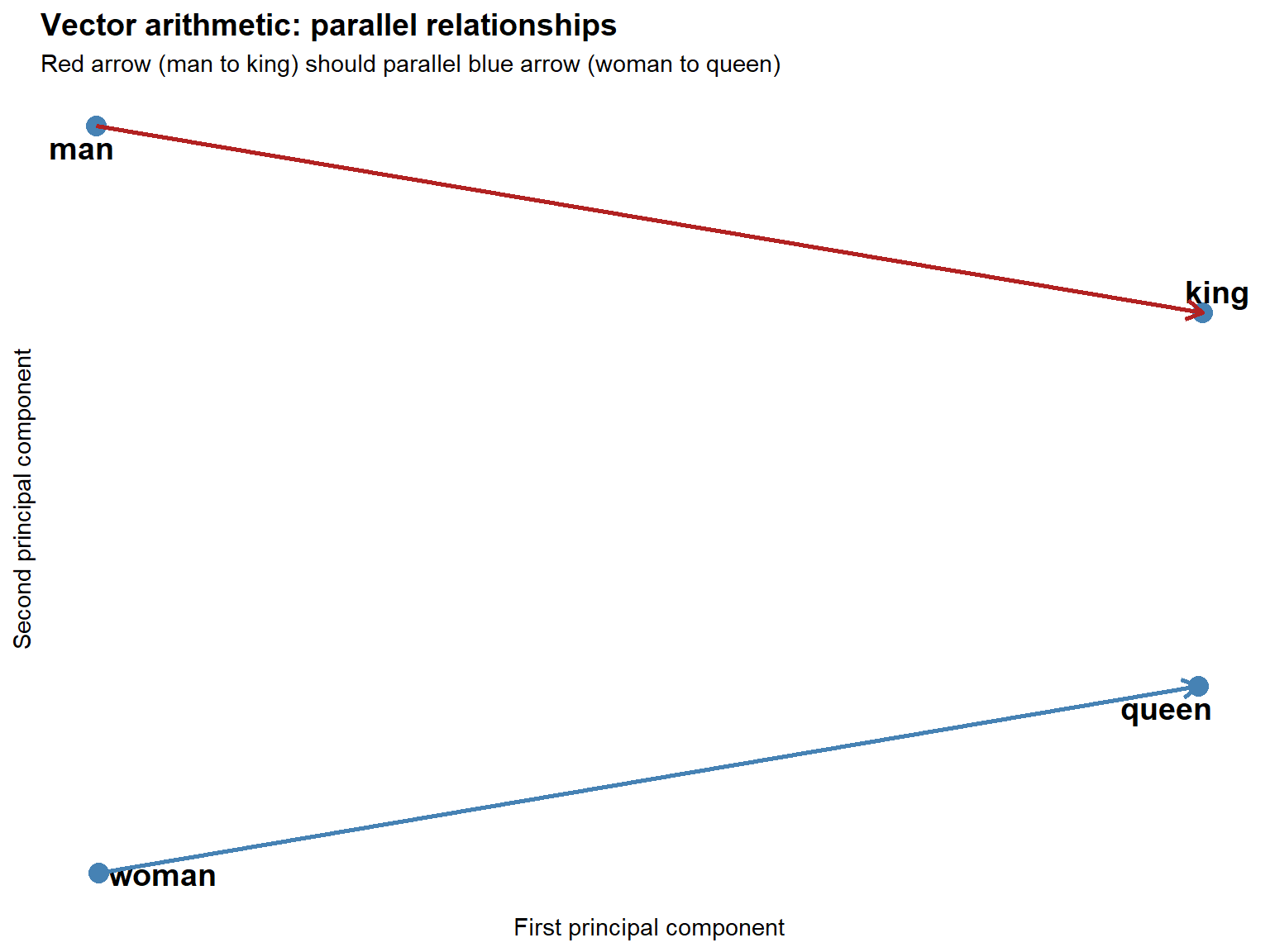
- Arrows should be roughly parallel and equal length
- This parallelism is what makes analogies work!

---

Part 6: Visualizing Embeddings

The Dimensionality Challenge

Problem: Embeddings have 50-300 dimensions. Humans visualize 2-3 dimensions.

Solution: Dimensionality reduction

• t-SNE (t-Distributed Stochastic Neighbor Embedding)
  
• UMAP (Uniform Manifold Approximation and Projection)
  
• PCA (Principal Component Analysis)

We’ll focus on t-SNE (most popular for embeddings).

t-SNE Visualization

Preparing Data

# Select interesting words to visualize  
words_to_plot <- c(  
  # Characters  
  "alice", "queen", "king", "hatter", "rabbit",  
  # Emotions  
  "happy", "sad", "angry", "joy", "fear",  
  # Actions    
  "walk", "run", "jump", "sit", "stand",  
  # Places  
  "house", "garden", "forest", "city", "ocean",  
  # Abstract  
  "love", "hate", "hope", "dream", "thought"  
)  
  
# Filter to words in vocabulary  
words_to_plot <- words_to_plot[words_to_plot %in% rownames(embedding_matrix)]  
  
# Get embeddings for these words  
plot_embeddings <- embedding_matrix[words_to_plot, ]  

Running t-SNE

# Set seed for reproducibility  
set.seed(42)  
  
# Run t-SNE  
tsne_result <- Rtsne(  
  plot_embeddings,  
  dims = 2,              # Reduce to 2 dimensions  
  perplexity = min(10, (nrow(plot_embeddings) - 1) / 3),  # Perplexity parameter  
  theta = 0.0,           # Exact t-SNE (slower but more accurate)  
  max_iter = 1000        # Iterations  
)  
  
# Create dataframe for plotting  
tsne_data <- data.frame(  
  word = words_to_plot,  
  x = tsne_result$Y[, 1],  
  y = tsne_result$Y[, 2],  
  # Add categories for coloring  
  category = case_when(  
    word %in% c("alice", "queen", "king", "hatter", "rabbit") ~ "Characters",  
    word %in% c("happy", "sad", "angry", "joy", "fear") ~ "Emotions",  
    word %in% c("walk", "run", "jump", "sit", "stand") ~ "Actions",  
    word %in% c("house", "garden", "forest", "city", "ocean") ~ "Places",  
    TRUE ~ "Abstract"  
  )  
)  

Creating the Visualization

ggplot(tsne_data, aes(x = x, y = y, color = category, label = word)) +  
  geom_point(size = 3, alpha = 0.7) +  
  geom_text_repel(  
    size = 4,  
    max.overlaps = 20,  
    box.padding = 0.5  
  ) +  
  scale_color_brewer(palette = "Set2") +  
  theme_minimal() +  
  theme(  
    legend.position = "bottom",  
    plot.title = element_text(size = 16, face = "bold"),  
    axis.text = element_blank(),  
    axis.ticks = element_blank(),  
    panel.grid = element_blank()  
  ) +  
  labs(  
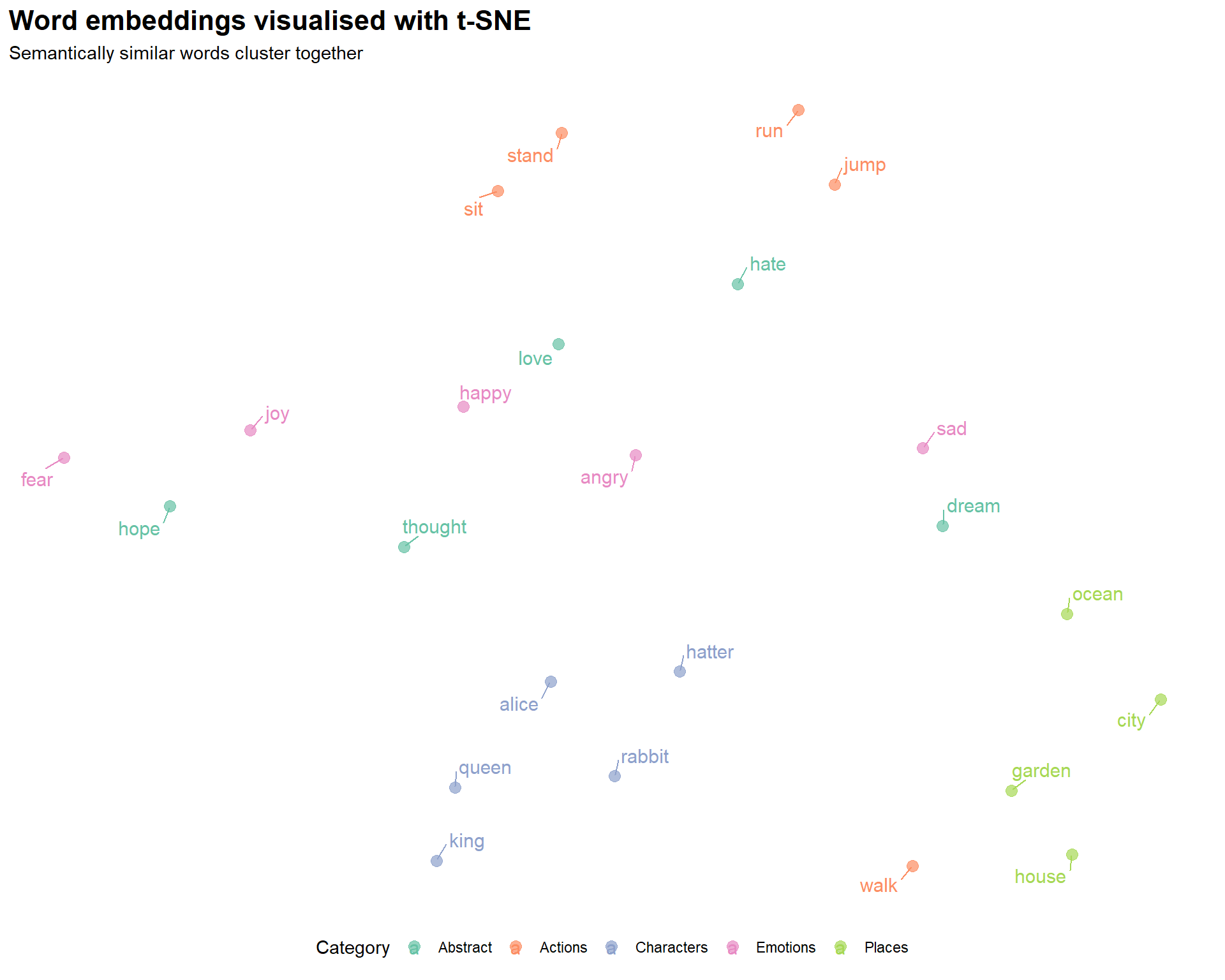
    title = "Word Embeddings Visualization (t-SNE)",  
    subtitle = "Semantically similar words cluster together",  
    x = NULL,  
    y = NULL,  
    color = "Category"  
  )  

Interpretation:
- Proximity = similarity: Words close together have similar meanings
- Clusters: Semantic categories group together
- Relative positions matter: Absolute coordinates are arbitrary

t-SNE Parameters

perplexity: Roughly how many neighbors to consider
- Too low: local structure overemphasized
- Too high: global structure lost
- Rule of thumb: 5-50, typically 30

iterations: How long to optimize
- More = better convergence
- 1000 often sufficient
- Watch for convergence in console output

theta: Speed/accuracy trade-off
- 0.0 = exact (slow, accurate)
- 0.5 = approximation (fast, good enough for large datasets)

---

Part 7: Using Pre-Trained Embeddings

Why Use Pre-Trained Models?

Advantages:
- ✅ Trained on massive datasets (billions of words)
- ✅ Better coverage of rare words
- ✅ No training time needed
- ✅ Validated quality
- ✅ Reproducible across studies

When to train your own:
- Specialized domain (medical, legal, historical)
- Unique vocabulary
- Limited pre-trained options for your language
- Research question requires custom training

GloVe Embeddings

GloVe (Global Vectors for Word Representation) is one of the most popular pre-trained embedding sets.

Downloading GloVe

# Download GloVe embeddings (one-time)  
library(textdata)  
  
# Download 100-dimensional GloVe vectors  
# Trained on 6 billion tokens from Wikipedia + Gigaword  
glove <- embedding_glove6b(dimensions = 100)  

# In practice, load pre-downloaded version  
# glove <- read.csv("path/to/glove.6B.100d.txt",   
#                   sep = " ", header = FALSE, quote = "")  
  
# For this tutorial, we'll simulate with our trained model  
# In your own work, use actual GloVe!  

Working with Pre-Trained Embeddings

# Structure: word in column 1, dimensions in remaining columns  
colnames(glove)[1] <- "word"  
colnames(glove)[2:ncol(glove)] <- paste0("dim_", 1:100)  
  
# Convert to matrix format for operations  
glove_matrix <- as.matrix(glove[, -1])  
rownames(glove_matrix) <- glove$word  
  
# Find similar words  
target_word <- "king"  
target_vector <- glove_matrix[target_word, ]  
  
# Calculate cosines with all words  
similarities <- apply(glove_matrix, 1, function(x) {  
  sum(x * target_vector) / (sqrt(sum(x^2)) * sqrt(sum(target_vector^2)))  
})  
  
# Top similar words  
head(sort(similarities, decreasing = TRUE), 10)  

Available Pre-Trained Models

Model	Size	Vocabulary	Dimensions	Use Case
GloVe	6B tokens	400K words	50-300	General purpose
fastText	600B tokens	2M words	300	Handles rare words, morphology
Word2Vec Google News	100B tokens	3M words	300	News domain
BERT	3.3B tokens	Contextual	768	Context-dependent tasks

Loading Different Models

# fastText (handles out-of-vocabulary words)  
library(fastrtext)  
model_ft <- load_model("path/to/fasttext/model.bin")  
  
# Word2Vec Google News  
library(wordVectors)  
model_gn <- read.vectors("GoogleNews-vectors-negative300.bin")  
  
# For transformers (BERT, RoBERTa, etc.)  
library(text)  # R interface to transformers  
# More complex setup - see dedicated transformer tutorials  

Choosing a Pre-Trained Model

GloVe:
- Simple, well-documented
- Good for general English
- Fast to load and use

fastText:
- Better for morphologically rich languages
- Handles misspellings and rare words
- Larger file sizes

BERT/Transformers:
- Context-dependent (different senses)
- State-of-the-art performance
- Requires more computational resources
- Use when context disambiguation critical

---

Part 8: Research Applications

Semantic Change Detection

Track how word meanings shift over time.

Comparing Embeddings Across Time

# Train separate models on different time periods  
corpus_1800s <- load_historical_corpus("1800-1850")  
corpus_1900s <- load_historical_corpus("1900-1950")  
corpus_2000s <- load_historical_corpus("2000-2020")  
  
model_1800s <- word2vec(corpus_1800s, dim = 100)  
model_1900s <- word2vec(corpus_1900s, dim = 100)  
model_2000s <- word2vec(corpus_2000s, dim = 100)  
  
# Compare word neighborhoods over time  
target_word <- "gay"  
  
# Get top neighbors in each period  
neighbors_1800s <- predict(model_1800s, target_word, type = "nearest")  
neighbors_1900s <- predict(model_1900s, target_word, type = "nearest")  
neighbors_2000s <- predict(model_2000s, target_word, type = "nearest")  
  
# Analyze shifting meanings  
# "gay" in 1800s: cheerful, happy  
# "gay" in 2000s: homosexual  

Research questions:
- When did semantic shift occur?
- What drove the change?
- Were there competing meanings?

Bias Detection

Uncover implicit associations in language.

Gender Bias Example

# Define gender direction  
man_vec <- embedding_matrix["man", ]  
woman_vec <- embedding_matrix["woman", ]  
gender_direction <- woman_vec - man_vec  
  
# Test occupations for gender bias  
occupations <- c("doctor", "nurse", "engineer", "teacher",   
                 "programmer", "secretary")  
  
occupation_bias <- sapply(occupations, function(occ) {  
  if (occ %in% rownames(embedding_matrix)) {  
    occ_vec <- embedding_matrix[occ, ]  
    # Project onto gender direction  
    sum(occ_vec * gender_direction) /   
      (sqrt(sum(occ_vec^2)) * sqrt(sum(gender_direction^2)))  
  } else {  
    NA  
  }  
})  
  
# Positive = more female-associated  
# Negative = more male-associated  
sort(occupation_bias)  

Findings from research:
- “Doctor”, “engineer” closer to “man”
- “Nurse”, “secretary” closer to “woman”
- Reflects societal biases in training data

Ethical Considerations

Embeddings encode biases from training data:
- Gender stereotypes
- Racial biases
- Cultural assumptions

Important for researchers:
- Acknowledge limitations
- Don’t amplify biases in applications
- Consider debiasing techniques
- Use diverse training data

Further reading:
- Bolukbasi et al. (2016). “Man is to Computer Programmer as Woman is to Homemaker?”
- Caliskan et al. (2017). “Semantics derived automatically from language corpora contain human-like biases”

Metaphor Analysis

Identify metaphorical mappings between domains.

Cross-Domain Associations

# Define source and target domains  
source_domain <- c("light", "bright", "illuminate", "shine", "glow")  
target_domain <- c("idea", "thought", "insight", "knowledge", "understanding")  
  
# Calculate cross-domain similarities  
metaphor_matrix <- matrix(0,   
                          nrow = length(source_domain),  
                          ncol = length(target_domain))  
  
rownames(metaphor_matrix) <- source_domain  
colnames(metaphor_matrix) <- target_domain  
  
for (i in 1:length(source_domain)) {  
  for (j in 1:length(target_domain)) {  
    s_word <- source_domain[i]  
    t_word <- target_domain[j]  
      
    if (s_word %in% rownames(embedding_matrix) &&   
        t_word %in% rownames(embedding_matrix)) {  
      # Cosine similarity  
      metaphor_matrix[i, j] <- sum(embedding_matrix[s_word,] *   
                                    embedding_matrix[t_word,]) /  
        (sqrt(sum(embedding_matrix[s_word,]^2)) *   
         sqrt(sum(embedding_matrix[t_word,]^2)))  
    }  
  }  
}  
  
# Visualize metaphorical connections  
library(pheatmap)  
pheatmap(metaphor_matrix,   
         main = "IDEAS ARE LIGHT metaphor",  
         display_numbers = TRUE)  

Research applications:
- Identify conventional metaphors
- Compare across languages
- Track metaphor evolution
- Study creative vs. conventional usage

Document Similarity

Average word embeddings to represent documents.

Document Vectors

# Function to create document embedding  
doc_to_vector <- function(doc_text, embedding_matrix) {  
  # Tokenize  
  words <- tolower(unlist(strsplit(doc_text, "\\s+")))  
    
  # Filter to vocabulary  
  words <- words[words %in% rownames(embedding_matrix)]  
    
  if (length(words) == 0) return(NULL)  
    
  # Average word vectors  
  doc_vec <- colMeans(embedding_matrix[words, ])  
  return(doc_vec)  
}  
  
# Apply to documents  
doc1_vec <- doc_to_vector(document1, embedding_matrix)  
doc2_vec <- doc_to_vector(document2, embedding_matrix)  
  
# Calculate similarity  
doc_similarity <- sum(doc1_vec * doc2_vec) /  
  (sqrt(sum(doc1_vec^2)) * sqrt(sum(doc2_vec^2)))  
  
cat("Document similarity:", doc_similarity)  

Applications:
- Find similar documents
- Cluster documents by topic
- Information retrieval
- Plagiarism detection

---

Part 9: Advanced Topics

Training Tips and Troubleshooting

Getting Better Embeddings

Data quality matters:

# More data is better (aim for 10M+ words for good results)  
# Clean data:  
corpus_clean <- corpus |>  
  # Lowercase (usually)  
  tolower() |>  
  # Fix encoding issues  
  iconv(to = "UTF-8") |>  
  # Normalize whitespace  
  str_replace_all("\\s+", " ") |>  
  # Handle URLs (remove or tag)  
  str_replace_all("http\\S+", "<URL>") |>  
  # Handle numbers (remove, tag, or keep)  
  str_replace_all("\\d+", "<NUM>")  

Hyperparameter tuning:

# Experiment systematically  
params_grid <- expand.grid(  
  dim = c(50, 100, 200),  
  window = c(5, 10, 15),  
  min_count = c(5, 10, 20)  
)  
  
# Train multiple models  
# Evaluate on analogy task or downstream application  
# Select best performing  

Common Problems and Solutions

Problem: “Training failed” error

Error: Training failed: fileMapper: [long text string]  

• ✓ Most common cause: Text not properly tokenized
  
• ✓ Solution: Split text into sentences/documents first
  
• ✓ Check: class(corpus) should be character vector, not single string
  
• ✓ Fix: Use str_split() or tokenize_sentences()

Example fix:

# WRONG: Single long string  
corpus <- paste(texts, collapse = " ")  
model <- word2vec(corpus)  # Will fail!  
  
# RIGHT: Vector of sentences  
corpus <- texts |>  
  paste(collapse = " ") |>  
  str_split("\\.\\s+") |>  
  unlist()  
model <- word2vec(corpus)  # Works!  

Problem: Poor quality results
- ✓ Increase corpus size (aim for 10M+ words)
- ✓ Clean data more thoroughly
- ✓ Adjust min_count (too high filters useful words)
- ✓ More training iterations (try 50+ for small corpora)
- ✓ Try different architecture (CBOW vs Skip-gram)

Problem: Out-of-vocabulary words
- ✓ Lower min_count
- ✓ Use fastText (handles subwords)
- ✓ Use pre-trained model with larger vocabulary

Problem: Slow training
- ✓ Reduce dimensions
- ✓ Smaller window size
- ✓ Negative sampling (already default)
- ✓ Use more CPU threads
- ✓ Consider text2vec package (faster)

Problem: Results not making sense
- ✓ Check data quality (garbage in = garbage out)
- ✓ Ensure corpus is large enough (minimum 1M words)
- ✓ Verify preprocessing didn’t remove too much
- ✓ Try different random seed
- ✓ Compare to baseline (pre-trained model)

Evaluation Methods

Intrinsic Evaluation

Word similarity datasets:

# WordSim-353, SimLex-999, etc.  
# Human-rated word pairs  
# Calculate correlation with embedding similarities  
  
evaluate_similarity <- function(model, test_pairs) {  
  model_scores <- sapply(1:nrow(test_pairs), function(i) {  
    predict(model,   
            newdata = c(test_pairs$word1[i], test_pairs$word2[i]),  
            type = "similarity")  
  })  
    
  cor(model_scores, test_pairs$human_score, method = "spearman")  
}  

Analogy datasets:

# Google analogy dataset  
# BATS (Bigger Analogy Test Set)  
# Measure accuracy: correct answer in top-n  
  
evaluate_analogies <- function(model, analogies) {  
  correct <- 0  
  total <- nrow(analogies)  
    
  for (i in 1:total) {  
    result <- predict(model,  
                     newdata = c(analogies$a[i], analogies$b[i], analogies$c[i]),  
                     type = "analogy",  
                     top_n = 5)  
      
    if (analogies$d[i] %in% result$term2) {  
      correct <- correct + 1  
    }  
  }  
    
  accuracy <- correct / total  
  return(accuracy)  
}  

Extrinsic Evaluation

Use in downstream tasks:
- Text classification accuracy
- Named entity recognition F1
- Sentiment analysis performance
- Information retrieval metrics

Best practice: Evaluate on your actual application!

Beyond Word2Vec

sentence2vec and doc2vec

Paragraph vectors:

library(doc2vec)  
  
# Train document embeddings  
model_doc <- paragraph2vec(  
  x = documents,  
  type = "PV-DBOW",  # Or PV-DM  
  dim = 100  
)  
  
# Get document vector  
doc_vec <- predict(model_doc, newdata = "new document text")  

When to use:
- Need document-level representations
- Variable-length inputs
- Document classification/clustering

Contextualized Embeddings (BERT, GPT)

The new frontier:

library(text)  
  
# BERT embeddings (context-dependent)  
embeddings <- textEmbed(  
  texts = c("The bank is near the river",  
            "I need to visit the bank"),  
  model = "bert-base-uncased"  
)  
  
# "bank" has DIFFERENT embeddings in these sentences!  

Advantages:
- Handles polysemy (multiple meanings)
- State-of-the-art performance
- Pre-trained on massive data

Disadvantages:
- Computationally expensive
- Requires GPU for speed
- More complex to work with
- Harder to interpret

Use contextualized when:
- Working with modern NLP tasks
- Polysemy is critical
- You have computational resources
- You need state-of-the-art performance

---

Part 10: Practical Workflow

Complete Analysis Pipeline

1. Decide on Approach

Decision tree:

Do you have domain-specific corpus?  
├─ YES: Should you train your own?  
│  ├─ Large corpus (10M+ words): Train custom  
│  └─ Small corpus: Use pre-trained + fine-tuning  
└─ NO: Use pre-trained embeddings  
   ├─ General English: GloVe  
   ├─ Rare words important: fastText  
   └─ Context crucial: BERT  

2. Prepare Data

# Full preprocessing pipeline  
preprocess_for_embeddings <- function(text,   
                                      lowercase = TRUE,  
                                      remove_punct = TRUE,  
                                      remove_numbers = FALSE,  
                                      min_word_length = 2) {  
    
  # Start with basic cleaning  
  clean_text <- text |>  
    # Fix encoding  
    iconv(to = "UTF-8", sub = "") |>  
    # Normalize whitespace  
    str_replace_all("\\s+", " ") |>  
    str_trim()  
    
  # Optional: lowercase  
  if (lowercase) {  
    clean_text <- tolower(clean_text)  
  }  
    
  # Optional: remove punctuation  
  if (remove_punct) {  
    clean_text <- str_replace_all(clean_text, "[^[:alnum:][:space:]]", " ")  
  }  
    
  # Optional: remove numbers  
  if (remove_numbers) {  
    clean_text <- str_replace_all(clean_text, "\\d+", "")  
  }  
    
  # Remove short words  
  if (min_word_length > 1) {  
    words <- unlist(strsplit(clean_text, "\\s+"))  
    words <- words[nchar(words) >= min_word_length]  
    clean_text <- paste(words, collapse = " ")  
  }  
    
  # Final normalization  
  clean_text <- str_squish(clean_text)  
    
  return(clean_text)  
}  

3. Train or Load Model

# Training workflow  
if (train_custom) {  
  # Prepare corpus  
  corpus <- preprocess_for_embeddings(raw_texts)  
    
  # Train with optimal parameters  
  model <- word2vec(  
    x = corpus,  
    type = "skip-gram",  
    dim = 100,  
    window = 5,  
    iter = 20,  
    min_count = 5,  
    threads = 4  
  )  
    
  # Save model  
  write.word2vec(model, "my_embeddings.bin")  
    
} else {  
  # Load pre-trained  
  embeddings <- load_pretrained_glove()  
}  

4. Apply to Research Question

# Example: Find specialized terminology  
find_domain_terms <- function(model, seed_terms, top_n = 50) {  
    
  # Get vectors for seed terms  
  seed_vectors <- embedding_matrix[seed_terms, ]  
    
  # Average to get domain centroid  
  domain_centroid <- colMeans(seed_vectors)  
    
  # Find nearest words  
  all_similarities <- apply(embedding_matrix, 1, function(x) {  
    sum(x * domain_centroid) /   
      (sqrt(sum(x^2)) * sqrt(sum(domain_centroid^2)))  
  })  
    
  # Return top matches  
  top_words <- names(sort(all_similarities, decreasing = TRUE)[1:top_n])  
    
  # Filter out seed terms  
  top_words <- setdiff(top_words, seed_terms)  
    
  return(top_words)  
}  
  
# Use it  
medical_seeds <- c("doctor", "patient", "hospital", "medicine")  
medical_terms <- find_domain_terms(model, medical_seeds)  

5. Validate and Interpret

# Validate results  
# 1. Manual inspection  
print(medical_terms[1:20])  # Do these make sense?  
  
# 2. Quantitative evaluation  
similarity_scores <- predict(model,   
                            newdata = medical_seeds,  
                            type = "nearest",  
                            top_n = 100)  
  
# 3. Visualize  
# Create t-SNE plot of domain  
# Compare to baseline/control words  
  
# 4. Statistical testing if applicable  
# Are similarities significantly different from random?  

Reproducibility Checklist

# Document everything  
analysis_metadata <- list(  
  date = Sys.Date(),  
  corpus_size = count_words(corpus),  
  preprocessing = list(  
    lowercase = TRUE,  
    remove_punct = TRUE,  
    min_count = 5  
  ),  
  model_params = list(  
    type = "skip-gram",  
    dim = 100,  
    window = 5,  
    iter = 20  
  ),  
  random_seed = 42,  
  package_versions = sessionInfo()  
)  
  
# Save metadata with model  
saveRDS(analysis_metadata, "model_metadata.rds")  
  
# Set seed for reproducibility  
set.seed(42)  
  
# Version control your code  
# git commit -m "Train embeddings with params X, Y, Z"  

---

Quick Reference

Essential Functions

# Training  
model <- word2vec(x = text, type = "skip-gram", dim = 100, window = 5)  
  
# Finding similar words  
similar <- predict(model, "king", type = "nearest", top_n = 10)  
  
# Word analogies  
analogy <- predict(model, c("king", "man", "woman"), type = "analogy")  
  
# Get embedding matrix  
embeddings <- as.matrix(model)  
  
# Save/load model  
write.word2vec(model, "model.bin")  
model <- read.word2vec("model.bin")  

Common Workflows

# Basic similarity analysis  
text |>  
  preprocess() |>  
  word2vec(dim = 100) -> model  
  
predict(model, "target_word", type = "nearest")  
  
# Visualization pipeline  
embeddings <- as.matrix(model)  
words_subset <- embeddings[selected_words, ]  
tsne_result <- Rtsne(words_subset, dims = 2)  
plot_tsne(tsne_result, labels = selected_words)  
  
# Custom research application  
semantic_shift <- compare_models(  
  model_period1,  
  model_period2,  
  target_words  
)  

---

Resources and Further Reading

Essential Papers

Foundational:
- Mikolov et al. (2013). “Efficient Estimation of Word Representations in Vector Space” (word2vec)
- Pennington et al. (2014). “GloVe: Global Vectors for Word Representation”
- Bojanowski et al. (2017). “Enriching Word Vectors with Subword Information” (fastText)

Applications:
- Hamilton et al. (2016). “Diachronic Word Embeddings Reveal Statistical Laws of Semantic Change”
- Bolukbasi et al. (2016). “Man is to Computer Programmer as Woman is to Homemaker?”
- Garg et al. (2018). “Word Embeddings Quantify 100 Years of Gender and Ethnic Stereotypes”

Reviews:
- Almeida & Xexéo (2019). “Word Embeddings: A Survey”

Books

• Jurafsky & Martin (2023). Speech and Language Processing (Chapter 6)
  
• Goldberg (2017). Neural Network Methods for Natural Language Processing
  
• Tunstall et al. (2022). Natural Language Processing with Transformers

Online Resources

Tutorials:
- Word2Vec Tutorial - The Skip-Gram Model
- Illustrated Word2vec
- GloVe: Global Vectors for Word Representation

Interactive:
- TensorFlow Embedding Projector
- Word2Viz

Datasets:
- Google Analogy Dataset
- WordSim-353
- SimLex-999

R Packages

Core:
- word2vec: User-friendly word2vec implementation
- text2vec: Fast, memory-efficient text analysis
- wordVectors: Load and manipulate embedding models

Related:
- textdata: Download pre-trained embeddings
- text: Interface to transformers (BERT, etc.)
- Rtsne: t-SNE dimensionality reduction
- umap: UMAP dimensionality reduction

---

Final Project Ideas

Capstone Projects

Apply what you’ve learned with these research projects:

1. Historical Semantic Change
- Collect texts from different decades
- Train separate embedding models
- Track meaning shifts of key terms
- Visualize changes over time

2. Domain-Specific Terminology
- Gather specialized corpus (medical, legal, technical)
- Train custom embeddings
- Extract domain vocabulary
- Compare to general English

3. Metaphor Mapping
- Identify source and target domains
- Calculate cross-domain similarities
- Visualize metaphorical connections
- Compare across languages/cultures

4. Bias Audit
- Load pre-trained embeddings
- Test for gender/racial biases
- Quantify stereotype associations
- Propose debiasing strategies

5. Document Clustering
- Represent documents as embedding averages
- Perform clustering analysis
- Validate against known categories
- Visualize document space

Deliverables:
- Documented R script
- Visualizations
- Brief report (1000 words)
- Interpretation of findings

---

Citation & Session Info

Schweinberger, Martin. 2026. Word Embeddings and Vector Semantics. Brisbane: The Language Technology and Data Analysis Laboratory (LADAL). url: https://ladal.edu.au/tutorials/embeddings.html (Version 2026.02.08).

@manual{schweinberger2026embeddings,  
  author = {Schweinberger, Martin},  
  title = {Word Embeddings and Vector Semantics},  
  note = {https://ladal.edu.au/tutorials/embeddings.html},  
  year = {2026},  
  organization = {The Language Technology and Data Analysis Laboratory (LADAL)},  
  address = {Brisbane},  
  edition = {2026.02.08}  
}  

Session Information

sessionInfo()  

R version 4.4.2 (2024-10-31 ucrt)
Platform: x86_64-w64-mingw32/x64
Running under: Windows 11 x64 (build 26200)

Matrix products: default


locale:
[1] LC_COLLATE=English_United States.utf8 
[2] LC_CTYPE=English_United States.utf8   
[3] LC_MONETARY=English_United States.utf8
[4] LC_NUMERIC=C                          
[5] LC_TIME=English_United States.utf8    

time zone: Australia/Brisbane
tzcode source: internal

attached base packages:
[1] stats     graphics  grDevices datasets  utils     methods   base     

other attached packages:
 [1] flextable_0.9.7 here_1.0.1      Rtsne_0.17      ggrepel_0.9.6  
 [5] ggplot2_3.5.1   purrr_1.0.4     tidyr_1.3.2     stringr_1.5.1  
 [9] dplyr_1.2.0     text2vec_0.6.4  word2vec_0.4.1 

loaded via a namespace (and not attached):
 [1] gtable_0.3.6            xfun_0.56               htmlwidgets_1.6.4      
 [4] lattice_0.22-6          vctrs_0.7.1             tools_4.4.2            
 [7] generics_0.1.3          tibble_3.2.1            pkgconfig_2.0.3        
[10] Matrix_1.7-2            data.table_1.17.0       RColorBrewer_1.1-3     
[13] uuid_1.2-1              lifecycle_1.0.5         compiler_4.4.2         
[16] farver_2.1.2            textshaping_1.0.0       munsell_0.5.1          
[19] RhpcBLASctl_0.23-42     codetools_0.2-20        fontquiver_0.2.1       
[22] fontLiberation_0.1.0    htmltools_0.5.9         yaml_2.3.10            
[25] pillar_1.10.1           crayon_1.5.3            openssl_2.3.2          
[28] rsparse_0.5.3           fontBitstreamVera_0.1.1 tidyselect_1.2.1       
[31] zip_2.3.2               digest_0.6.39           stringi_1.8.4          
[34] labeling_0.4.3          rprojroot_2.0.4         fastmap_1.2.0          
[37] grid_4.4.2              colorspace_2.1-1        cli_3.6.4              
[40] magrittr_2.0.3          withr_3.0.2             gdtools_0.4.1          
[43] scales_1.3.0            float_0.3-2             rmarkdown_2.30         
[46] officer_0.6.7           mlapi_0.1.1             askpass_1.2.1          
[49] ragg_1.3.3              evaluate_1.0.3          knitr_1.51             
[52] rlang_1.1.7             Rcpp_1.0.14             glue_1.8.0             
[55] xml2_1.3.6              renv_1.1.1              rstudioapi_0.17.1      
[58] jsonlite_1.9.0          lgr_0.4.4               R6_2.6.1               
[61] systemfonts_1.2.1      

---

Back to top

Back to HOME

---

References

Almeida, F., & Xexéo, G. (2019). Word embeddings: A survey. arXiv preprint arXiv:1901.09069.

Bojanowski, P., Grave, E., Joulin, A., & Mikolov, T. (2017). Enriching word vectors with subword information. Transactions of the Association for Computational Linguistics, 5, 135-146.

Bolukbasi, T., Chang, K. W., Zou, J. Y., Saligrama, V., & Kalai, A. T. (2016). Man is to computer programmer as woman is to homemaker? Debiasing word embeddings. Advances in Neural Information Processing Systems, 29.

Firth, J. R. (1957). A synopsis of linguistic theory, 1930-1955. Studies in Linguistic Analysis, 1-32.

Garg, N., Schiebinger, L., Jurafsky, D., & Zou, J. (2018). Word embeddings quantify 100 years of gender and ethnic stereotypes. Proceedings of the National Academy of Sciences, 115(16), E3635-E3644.

Goldberg, Y. (2017). Neural network methods for natural language processing. Morgan & Claypool Publishers.

Hamilton, W. L., Leskovec, J., & Jurafsky, D. (2016). Diachronic word embeddings reveal statistical laws of semantic change. Proceedings of the 54th Annual Meeting of the Association for Computational Linguistics, 1489-1501.

Jurafsky, D., & Martin, J. H. (2023). Speech and language processing (3rd ed. draft). https://web.stanford.edu/~jurafsky/slp3/

Mikolov, T., Chen, K., Corrado, G., & Dean, J. (2013). Efficient estimation of word representations in vector space. arXiv preprint arXiv:1301.3781.

Pennington, J., Socher, R., & Manning, C. D. (2014). GloVe: Global vectors for word representation. Proceedings of the 2014 Conference on Empirical Methods in Natural Language Processing, 1532-1543.

Tunstall, L., von Werra, L., & Wolf, T. (2022). Natural language processing with transformers. O’Reilly Media.

References

Almeida, Felipe, and Geraldo Xexéo. 2019. “Word Embeddings: A Survey.” https://doi.org/10.48550/arXiv.1901.09069.
Bojanowski, Piotr, Edouard Grave, Armand Joulin, and Tomas Mikolov. 2017. “Enriching Word Vectors with Subword Information.” Transactions of the Association for Computational Linguistics 5: 135–46. https://doi.org/10.1162/tacl_a_00051.
Bolukbasi, Tolga, Kai-Wei Chang, James Y. Zou, Venkatesh Saligrama, and Adam Tauman Kalai. 2016. “Man Is to Computer Programmer as Woman Is to Homemaker? Debiasing Word Embeddings.” In Advances in Neural Information Processing Systems 29 (NeurIPS 2016), 4349–57. Barcelona, Spain. https://proceedings.neurips.cc/paper/2016/hash/a486cd07e4ac3d270571622f4f316ec5-Abstract.html.
Caliskan, Aylin, Joanna J. Bryson, and Arvind Narayanan. 2017. “Semantics Derived Automatically from Language Corpora Contain Human-Like Biases.” Science 356 (6334): 183–86. https://doi.org/10.1126/science.aal4230.
Firth, John R. 1957. “A Synopsis of Linguistic Theory, 1930–1955.” In Studies in Linguistic Analysis, 1–32. Oxford: Blackwell.
Garg, Nikhil, Londa Schiebinger, Dan Jurafsky, and James Zou. 2018. “Word Embeddings Quantify 100 Years of Gender and Ethnic Stereotypes.” Proceedings of the National Academy of Sciences 115 (16): E3635–44. https://doi.org/10.1073/pnas.1720347115.
Goldberg, Yoav. 2017. Neural Network Methods for Natural Language Processing. Synthesis Lectures on Human Language Technologies 37. Morgan & Claypool Publishers. https://doi.org/10.2200/S00762ED1V01Y201703HLT037.
Hamilton, William L., Jure Leskovec, and Dan Jurafsky. 2016. “Diachronic Word Embeddings Reveal Statistical Laws of Semantic Change.” In Proceedings of the 54th Annual Meeting of the Association for Computational Linguistics (Volume 1: Long Papers), 1489–1501. Berlin, Germany: Association for Computational Linguistics. https://doi.org/10.18653/v1/P16-1141.
Jurafsky, Daniel, and James H. Martin. 2024. Speech and Language Processing: An Introduction to Natural Language Processing, Computational Linguistics, and Speech Recognition. Third Edition (draft). https://web.stanford.edu/~jurafsky/slp3/.
Mikolov, Tomas, Kai Chen, Greg Corrado, and Jeffrey Dean. 2013. “Efficient Estimation of Word Representations in Vector Space.” In Proceedings of the 1st International Conference on Learning Representations (ICLR 2013), Workshop Track. Scottsdale, AZ. https://doi.org/10.48550/arXiv.1301.3781.
Pennington, Jeffrey, Richard Socher, and Christopher D. Manning. 2014. “GloVe: Global Vectors for Word Representation.” In Proceedings of the 2014 Conference on Empirical Methods in Natural Language Processing (EMNLP), 1532–43. Doha, Qatar: Association for Computational Linguistics. https://doi.org/10.3115/v1/D14-1162.
Tunstall, Lewis, Leandro von Werra, and Thomas Wolf. 2022. Natural Language Processing with Transformers. Revised. Sebastopol, CA: O’Reilly Media.